Estimate peak air-gap flux density. Compare geometry and single or dual rotors, then check the model limits before selecting magnets.
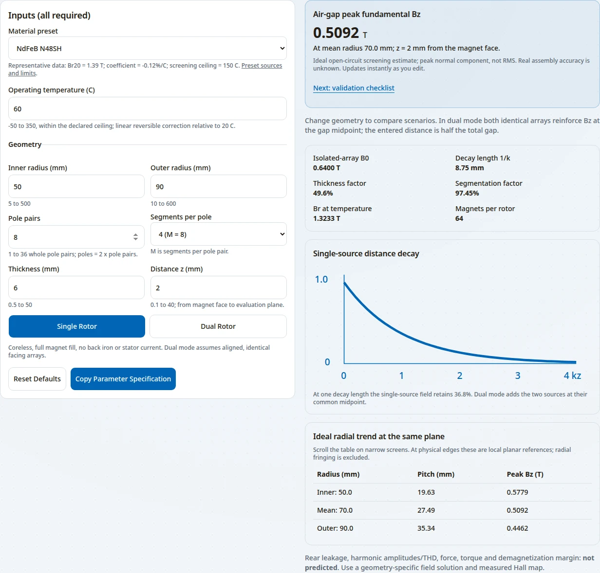
Air-gap peak fundamental Bz
0.5092 T
At mean radius 70.0 mm; z = 2 mm from the magnet face.
Ideal open-circuit screening estimate; peak normal component, not RMS. Real assembly accuracy is unknown. Default estimate; JavaScript enables editing.
Change geometry to compare scenarios. In dual mode both identical arrays reinforce Bz at the gap midpoint; the entered distance is half the total gap.
Inputs (all required)
Isolated-array B0 0.6400 T
Decay length 1/k 8.75 mm
Thickness factor 49.6%
Segmentation factor 97.45%
Br at temperature 1.3233 T
Magnets per rotor 64
Single-source distance decay
At one decay length the single-source field retains 36.8%. Dual mode adds the two sources at their common midpoint.
Ideal radial trend at the same plane
Scroll the table on narrow screens. At physical edges these are local planar references; radial fringing is excluded.
Local planar fundamental at inner, mean and outer radius
Radius (mm)
Pitch (mm)
Peak Bz (T)
Inner: 50.0
19.63
0.5779
Mean: 70.0
27.49
0.5092
Outer: 90.0
35.34
0.4462
Rear leakage, harmonic amplitudes/THD, force, torque and demagnetization margin: not predicted. Use a geometry-specific field solution and measured Hall map.
First recorded: · Reviewed: · Sources checked: October 27, 2026 · Next review: April 27, 2027
Prepared and maintained by Halbach Array, a commercial magnetic assembly supplier. We may quote assemblies discussed here. The first recorded date is the repository record; public publication has not been independently verified. Calculated examples are software evidence, not customer results or hardware qualification.
1. Conclusions you can use
Decision summary: estimates, evidence and the next check · Scroll horizontally on small screens.
Check actual hot B-H curves and reverse-field load cases.
2. Reproduce the estimate
The tool applies a local planar fundamental model to an annulus. The planar amplitude and decay follow Post and Ryutov; replacing the linear wavenumber with p/r is the approximation made on this page. It assumes uniform equal-angle segments, full fill, no iron, no current and magnet relative recoil permeability of one.
r_mean = (R_in + R_out) / 2; k = p / r_mean; pole pitch = pi / k
M = 2 * segments_per_pole; S = sin(pi/M) / (pi/M)
Br(T) = Br20 * [1 + alpha * (T - 20) / 100]
B0 = Br(T) * S * [1 - exp(-k*h)]
Single: Bz(z) = B0 * exp(-k*z)
Dual: Bz(s) = B0 * [exp(-k*s) + exp(-k*(g-s))]
Dual midpoint: s = z = g/2; Bz = 2 * B0 * exp(-k*z)
Use mm for every length so k is in inverse mm; the exponents remain dimensionless. The result is the angular peak of the normal fundamental at the selected radius and plane. B0 always refers to an isolated array; it is not the total surface field of the dual assembly.
With the defaults: Br20 = 1.39 T, alpha = -0.12%/C, T = 60 C, radii 50/90 mm, p = 8, M = 8, h = 6 mm and z = 2 mm, the model gives Br(T) = 1.3233 T, B0 = 0.6400 T and Bz = 0.5092 T.
Original software run captured October 27, 2026, with the defaults above: single rotor, four segments per pole (M = 8), declared ceiling 150 C, Bz = 0.5092 T. Sticky navigation and floating contact are hidden only in this isolated capture. This is a reproducible calculator result, not a measured magnet test, customer endorsement or assembly qualification.
3. Distance, pitch and diminishing thickness returns
Compare dimensionless ratios before changing a design. At fixed Br and segmentation, distance multiplies the field by exp(-kz), while thickness multiplies it by 1-exp(-kh). These factors are calculated from the equations above; they are not measured machine efficiencies.
Reproducible normalized factors; pole pitch = pi/k · Scroll horizontally on small screens.
Ratio
Distance retained at z/pitch
Thickness factor at h/pitch
0.1
73.0%
27.0%
0.25
45.6%
54.4%
0.5
20.8%
79.2%
1
4.3%
95.7%
Going from h = 0.5 pitch to h = 1.0 pitch raises the thickness factor from 79.2% to 95.7%: 16.5 percentage points, or about 20.8% relative field gain. Magnet volume doubles at unchanged planform. A cost increase needs a supplier quote; it cannot be inferred from volume alone.
4. Segmentation: fundamental gain and what remains unknown
The equal-step fundamental factor approaches one as M rises. The planar report supports this screening factor; a full harmonic solution needs the actual magnetization and observation region. The tool does not infer a total harmonic distortion from two selected sidebands.
Calculated equal-step factors and per-rotor part counts for eight pole pairs · Scroll horizontally on small screens.
Segments / pole
M / pole pair
Fundamental factor
Magnets / rotor
2
4
90.03%
32
3
6
95.49%
48
4
8
97.45%
64
6
12
98.86%
96
8
16
99.36%
128
Choose segmentation against the waveform requirement, available magnetization directions, bond lines, inspection and assembly cost. A higher factor alone does not establish low eddy-current loss or low machine torque ripple. Rear leakage remains unknown without finite geometry and a measurement plane.
5. Single and dual arrays: compare the same plane
Both sources are evaluated at the same plane. Phase, gap definition and reference B0 must match.
Topology tradeoffs under the free-space, coreless assumptions · Scroll horizontally on small screens.
Question
Single array
Matched dual arrays
Field at distance z
B0 * exp(-kz)
2 * B0 * exp(-kz) at midpoint; g = 2z
Magnet inventory
One rotor
Two identical rotors; twice the magnet count
Mechanical review
Retention and any loads from surrounding material
Rotor-to-rotor attraction, disc deflection and assembly fixturing
When the simple comparison fails
Iron, current, edge fringing or partial fill
All single-array limits plus phase mismatch or unequal arrays
Symmetry does not remove rotor attraction. Evaluate force using the full field and a defined integration surface, then check discs, bearings, retention and fault loads. The force calculation guide explains the separate force task.
6. Material and temperature inputs
These presets are representative supplier catalog inputs, checked October 27, 2026. Br refers to 20 C; coefficients are in percent per C. A listed maximum is a screening ceiling, not an assembly qualification. Supplier ranges, product revisions and actual B-H curves take precedence.
Transparent calculator presets; no hot coercivity or safe-load-line values are inferred · Scroll horizontally on small screens.
The reversible correction uses the signed temperature difference, including below 20 C. It is only a linear approximation over a supplier-supported range. Coercivity and irreversible losses are not calculated. Enter a custom material when its Br, coefficient or documented ceiling differs.
For demagnetization review, obtain temperature-dependent curves and check local operating points against worst-case reverse fields. IEC 60404-5 describes material measurement scope; IEC 60404-8-1:2023 covers material specifications. Neither proves that this assembly is safe at the catalog ceiling.
7. Model limits, risks and alternatives
This calculator adapts a planar fundamental. It does not solve the finite annulus. Xia, Zhu and Howe show the importance of material and boundary conditions in cylindrical machines; Okita and Harada provide an axial-specific 3D treatment. Those papers do not give this tool a universal error percentage.
Known outputs and unresolved quantities · Scroll horizontally on small screens.
Quantity or risk
Status here
Minimum next step
Peak fundamental and geometry trends
Calculated under the displayed assumptions
Match peak/RMS convention, radius, angular location and probe plane.
Radial edge field and finite-geometry error
Unknown; no calibrated correction
Model finite sectors and scan across the radial span.
Rear leakage and spatial THD
Unknown; fundamental only
Specify rear probe distance; solve and measure the full waveform.
Hot demagnetization / fault current
Not calculated
Use hot supplier curves, local working points and current load cases.
Torque, force and mechanical safety
Not calculated
Use full-field stress integration and mechanical load analysis.
Manufacturing cost and assembly yield
Unknown without a quote
Request segmented-part, tooling, fixture and inspection costs.
Slotted or iron-cored machine fit
Outside the free-space assumptions
Include nonlinear materials, slots, windings and armature reaction.
A narrow annulus, few pole pairs or large radial span can weaken the planar approximation. A 3D magnetic model with mesh convergence and measurement comparison is the practical alternative. More decimal places in the calculator do not establish greater physical accuracy.
8. Three reproducible design comparisons
These are calculated examples using the displayed equations, not customer case studies, simulations or measured performance. Each starts from the default N48SH inputs: 50/90 mm radii, eight pole pairs, M = 8, 60 C, 6 mm thickness and 2 mm distance.
Increase the evaluation distance
Single array; change z from 2 to 4 mm.
0.4051 T
Baseline 0.5092 T; change -20.4%.
Keep structural clearance requirements, then compare the loss against the field target. Do not reduce a clearance solely to recover field.
Add a matched second rotor
Two identical reinforcing arrays; total gap g = 4 mm, midpoint z = 2 mm.
1.0184 T
Baseline 0.5092 T; change 100.0%.
The ideal midpoint field doubles relative to a single source at the same distance. Review rotor attraction, alignment and assembly fixtures before selecting this topology.
Compare thicker magnets
Single array; change thickness from 6 to 12 mm at fixed z = 2 mm.
0.7657 T
Baseline 0.5092 T; change 50.4%.
Compare this incremental field gain with magnet volume, rotor mass, retention and supplier pricing. The tool does not predict machine efficiency or torque.
9. From a screening result to a field acceptance plan
Agree the comparison quantity before comparing solver results and measurements.
Record the magnet geometry, orientation sequence, bond lines, material curves, total gap and actual evaluation plane. Specify peak, RMS or pole-average convention.
Include surrounding ferromagnetic and conductive parts, temperature and relevant current cases in the magnetic model. Check mesh convergence and local reverse fields; do not use a fixed generic fringing discount.
Agree Hall-probe radii, angular samples, axial standoff, calibration, orientation and temperature. Sample densely enough to resolve the waveform of interest, then check convergence by increasing sample density.
Compare fundamental amplitude and full waveform at identical coordinates. Record uncertainty and tolerances. Material characterization and assembled-rotor field mapping answer different questions.
If the calculator rejects the geometry, document those same inputs and request a geometry-specific solution. This provides a usable next step without extrapolating the tool outside its ranges.
The answers use the assumptions, equations and linked sources above. They do not replace a machine-specific field and load analysis.
Equations and measurement
What does the axial Halbach array magnetic field calculator return?
The peak fundamental normal flux density Bz at the mean radius and specified plane. It is a local planar, open-circuit estimate with full magnet fill and relative recoil permeability set to one. It is not RMS, pole-average field, torque or a certified field map.
What is the fundamental field equation?
For one array, B0 = Br(T) * sin(pi/M)/(pi/M) * (1 - exp(-k*h)), and Bz(z) = B0 * exp(-k*z). The local wavenumber is k = p/r, with pole pairs p, radius r and M segments per pole pair. Use consistent length units.
How is the dual-rotor midpoint calculated?
Two identical arrays phased to reinforce the normal field add at the same plane: Bz(s) = B0 * [exp(-k*s) + exp(-k*(g-s))]. At s = g/2 the result is 2*B0*exp(-k*g/2). Enter z = g/2 in dual mode. Iron and load-current effects are excluded.
Is distance z the whole mechanical gap?
For a single array, z is magnet-face-to-evaluation-plane distance. For dual arrays, z is half the total face-to-face separation g = 2z. Include winding, encapsulation and clearance when locating the plane; do not enter just rotor-to-stator clearance.
Why is the result labeled peak fundamental rather than field strength?
Flux density B is measured in tesla; magnetic field strength H is measured in A/m. This estimate describes the amplitude of the normal fundamental component. Comparing it with probe readings requires matching the radius, plane and angular peak.
Does the tool predict the true field at inner and outer edges?
No. The radial table changes the local pole pitch with radius, but omits finite-edge fringing. Inner and outer rows are ideal trend references. Use 3D analysis and a radial Hall scan for physical edge values.
Geometry and design tradeoffs
Why does the field decrease with distance?
In the source-free planar model each spatial Fourier component decays with distance. The fundamental retains exp(-k*z); at z = 1/k it retains 36.8% of its isolated-array surface amplitude. Radial edge effects can change real measurements.
Does more magnet thickness always give proportionally more field?
No. The thickness factor is 1-exp(-k*h). Doubling h from half a pole pitch to one pole pitch increases this factor from 79.2% to 95.7%, a relative field increase of about 20.8% at fixed geometry and Br. This is a calculated trend, not a cost quote.
Is more segmentation always better?
More equal magnetization steps raise the ideal fundamental factor toward one. M=4 gives 90.03%, M=8 gives 97.45%, and M=16 gives 99.36%. Additional magnets also add placement, bonding and inspection work; decide using a quoted assembly and measured field target.
Can the tool calculate spatial THD or rear leakage?
No. A fundamental-only model does not determine a complete harmonic spectrum or finite-rotor rear leakage. Those require specified magnetization, clearances, geometry and a field solution or measurement. No universal shielding ratio is assumed.
Can I use the estimate with back iron or a slotted stator?
Use it only as a free-space screening reference. Iron permeability, saturation, slot geometry and armature reaction alter the boundary conditions. Use a model that includes those materials and currents before making an acceptance decision.
Do dual rotors eliminate axial mechanical loads?
No. Symmetry can reduce net stator force in an ideal arrangement, while the rotors still attract each other. Size retention, discs and bearings with a geometry-specific stress calculation, assembly load cases and mechanical analysis.
Materials and verification
How does the temperature correction work?
Br(T) = Br20 * [1 + alpha*(T-20)/100], where alpha is entered in percent per C. The signed correction also applies below 20 C, with an extrapolation warning. It represents reversible change only and requires supplier confirmation over the actual temperature range.
Does staying below a preset temperature ceiling guarantee no demagnetization?
No. Reverse field, operating point, temperature-dependent B-H curves and transient current all matter. The ceiling is only a screening input. Check local magnet operating points for the worst thermal and electrical load cases.
How should I enter a custom material?
Supply Br at 20 C, its reversible temperature coefficient and a documented temperature ceiling. Those fields stay visible alongside operating temperature. Replace the prefilled screening assumptions with the actual supplier data.
When should I compare SmCo with NdFeB?
Compare specific documented grades when reversible temperature stability or hot operation matters. Use the table as a starting point; coercivity, operating point, corrosion protection, mechanical strength and procurement conditions still need separate review.
How should a manufactured array be checked?
Define a calibrated Hall-probe scan at agreed radii, angular positions and axial planes, recording temperature, probe orientation, standoff and uncertainty. Compare the fundamental and full waveform with 3D predictions; request supplier material curves separately.
What should I send for a field review or quotation?
Send radii, pole pairs, segments and magnetization directions, thickness, total separation and probe plane, material curves, target peak or RMS convention, operating temperatures, surrounding materials, current load cases, retention details and quantity.
11. Traceable sources and evidence limits
Publication records and public catalog scopes checked October 27, 2026. The page uses the cited scope shown below; numerical comparisons are analytical calculations, not claimed measurements. Unavailable or unverified hardware outcomes remain unknown.
R. F. Post and D. D. Ryutov, Lawrence Livermore National Laboratory · 2000
Primary report describing the planar Halbach fundamental, exponential distance decay and segmentation factor. Applying k = p/r to an annulus here is a local planar approximation, not a 3D solution.
J. C. Mallinson, IEEE Transactions on Magnetics 9(4), 678–682 · 1973
Foundation for one-sided flux distributions under ideal magnetization conditions. It does not establish a rear leakage allowance for a finite manufactured rotor.
K. Halbach, Nuclear Instruments and Methods 169(1), 1–10 · 1980
Foundational oriented permanent multipoles; background for magnetization design, not validation of this calculator or an axial machine performance guarantee.
Z. P. Xia, Z. Q. Zhu and D. Howe, IEEE Transactions on Magnetics 40(4), 1864–1872 · 2004
Polar-coordinate models include recoil permeability and compare with FEA and measurements. Its internal/external rotor analysis should not be read as an axial-annular error bound.
T. Okita and H. Harada, IEEE Access 11, 2078–2091 · 2023
Axial-machine-specific 3D formulation illustrates why finite geometry needs its own field model. No universal radial correction percentage is inferred from it here.
Arnold Magnetic Technologies · Live manufacturer catalog; checked October 27, 2026
RECOMA 30S sheet, PDF page 14: nominal Br 1.12 T, coefficient -0.035%/C measured between 20 and 150 C, listed ceiling 350 C. The ceiling does not validate linear extrapolation to 350 C.
International Electrotechnical Commission, TC 68 · 2015
Official public scope covers flux density, polarization, field strength, demagnetization curves and recoil lines. This page does not claim to reproduce or certify the paid standard.
International Electrotechnical Commission, TC 68 · 2023
Current cataloged edition replaces the 2015 material specification. Its scope covers principal properties and dimensional tolerances, not guaranteed operating limits of an assembled rotor.
Copy the tool specification and include the target field convention, probe plane, temperature-dependent material curves, surrounding materials and current cases. Confirm the required simulation, mapping and acceptance scope with the engineering team.